
Database technologies have undergone significant diversification in recent years. Now we encounter specialized solutions for every data type and usage scenario. In this rich ecosystem, optimized systems for time series data stand out in particular. One of the most notable solutions in this field is TigerData, formerly known as TimescaleDB.
TimescaleDB now continues as Tigerdata. Although the name has changed, the strong time series data architecture, PostgreSQL compatibility, and scalability features remain the same. In this article, we will explain both what this transformation means and why Tigerdata is still one of the most powerful solutions.
What is TigerData?
Time series data has become a crucial part of today’s applications and systems. Various data types, such as measurements from IoT devices, financial market data, user interactions, and system logs, are recorded over time. Traditional relational databases are usually inadequate for storing, querying, and analyzing this kind of data. That’s where TigerData comes into play.
An Application With TigerData
As the article continues, we will exemplify through the application while talking about the features of Tigerdata.
For your performance comparisons before starting the application, Tigerdata 4 core CPU (AMD Ryzen 5 3600 6 Core), 32GB Memory, 200GB NVME features on the Rocky Linux operating system.
We downloaded the “Top Cryptocurrencies Prices” dataset via Kaggle. It contains cryptocurrency price values at data-minute intervals. (Source: https://www.kaggle.com/datasets/prasertk/top-cryptocurrencies-prics-minute-interval?Resource=download)
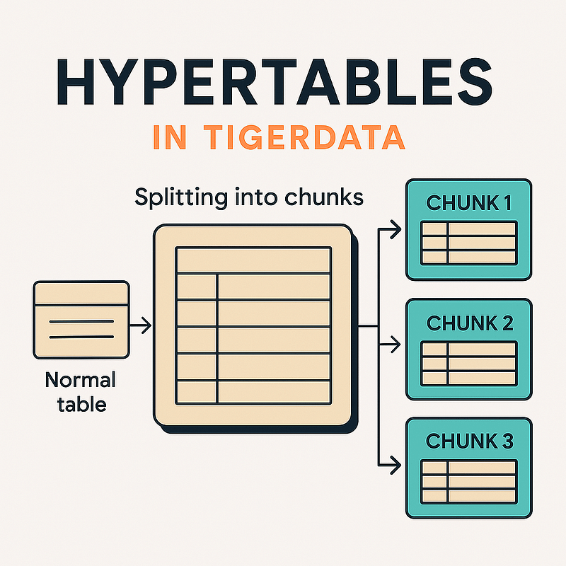
What is Hypertable?
Hypertable automatically divides data into pieces according to time intervals (optionally compared to other columns). These parts are physically separate in sub-sections called “chunks”. For the user, the table still appears to be one piece, while the system in the background performs data writing, inquiry, and compression processes in a much more performance way.
How is Hypertable’s Time Interval Determined? (chunk_time_interval)
If you do not specify any period in TigerData, chunks are set to 1 week by default. However, for optimal performance, it is recommended that 1 chunk should be a maximum of 25% of the memory size on your server. For example, our server has 32GB of RAM. Therefore, the size of 1 chunk should be approximately 8GB. If the data we have generates 1GB of data on a daily basis, we will have 7GB of data in 7 days, so the chunk can be determined as 7 days. This means that one chunk table will be created every 7 days. If it generates 16GB of data in a day, the chunk should be set to half a day. However, this setting can be changed according to the intended use.
We first insert some of the data into a normal table. After looking at the size of this table, we look at how many days are in the sample table.
Now it’s time to create HYPERTABLE!!!
Learning the table size:
SELECT
    schemaname || '.' || relname AS table_name,
    pg_size_pretty(pg_total_relation_size(relid)) AS total_size,
    pg_size_pretty(pg_relation_size(relid)) AS table_size,
    pg_size_pretty(pg_total_relation_size(relid) - pg_relation_size(relid)) AS index_size
FROM
    pg_catalog.pg_statio_user_tables
where schemaname = 'schema_name' and relname = 'table_name'
ORDER BY
pg_total_relation_size(relid) DESC;To observe how many days are included in the sample data:
select max(transaction_time)- min(transaction_time)
from tmp_schema.coin_dataIt may also be useful to look at the normality distribution of the number of rows of data in a day:
select time_bucket('1 day',transaction_time), count(*)
from tmp_schema.coin_data
group by 1Based on this information, the chunk_time_interval value can be determined. Mathematically, we can formulate it as follows:
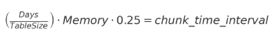
The size of our table is about 2.3GB. The data that provides this size is 828 days old. Under normal circumstances, chunk_time_interval should be given in larger intervals, but since it is a sample study, we will specify a 1-week chunk_time_interval.
Creating table
CREATE TABLE tmp_schema.coin_data (
 transaction_time timestamp NULL,
 symbol varchar(15) NULL,
 open_value float4 NULL,
 high_value float4 NULL,
 low_value float4 NULL,
 close_value float4 NULL,
 volume_coin float4 NULL,
 volume_usdt float8 NULL,
 trade_count int4 NULL
);SELECT create_hypertable('tmp_schema.coin_data', by_range('transaction_time', INTERVAL '1 week'));If there is data in the table
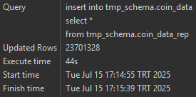
SELECT create_hypertable('tmp_schema.coin_data', by_range('transaction_time', INTERVAL '1 week'),migrate_data => true);We inserted the previously stored data from the regular table into the hypertable.
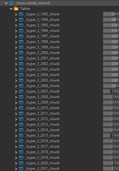
The chunk tables are stored in the _timescaledb_internal schema. In the image below, we see that the chunk tables are created.
Which Chunk Belongs to Which Table?!!!!
I realize that you are asking this question for large buildings with many tables, and the answer is very simple
SELECT show_chunks('tmp_schema.coin_data');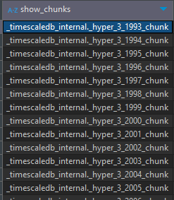
What if I want to change the chunk_time_interval later?
After creating the table and setting the chunk_time_interval value, if you want to change this interval, there is a simple solution.
SELECT set_chunk_time_interval('tmp_schema.coin_data', INTERVAL '6 month');Ease of Select with Hypertable
One of the best features of Hypertable is the ease of typing when querying time series.
Examples:
select time_bucket('1 year',transaction_time) as transaction_year,
symbol as coin_name, round(avg(open_value)::numeric,2) as avg_open_value
from tmp_schema.coin_data
where symbol = 'BTC/USDT'
group by 1,2
order by 1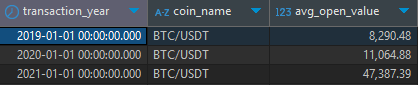
select time_bucket('1 day',transaction_time) as transaction_year,
symbol as coin_name, round(avg(open_value)::numeric,2) as avg_open_value,
round(avg(close_value)::numeric,2) as avg_close_value,
round(avg((high_value+low_value)/2)::numeric,2) as avg_value_high_low
from tmp_schema.coin_data
where time_bucket('1 year',transaction_time) between '2020-01-01' and '2021-01-01'
group by 1,2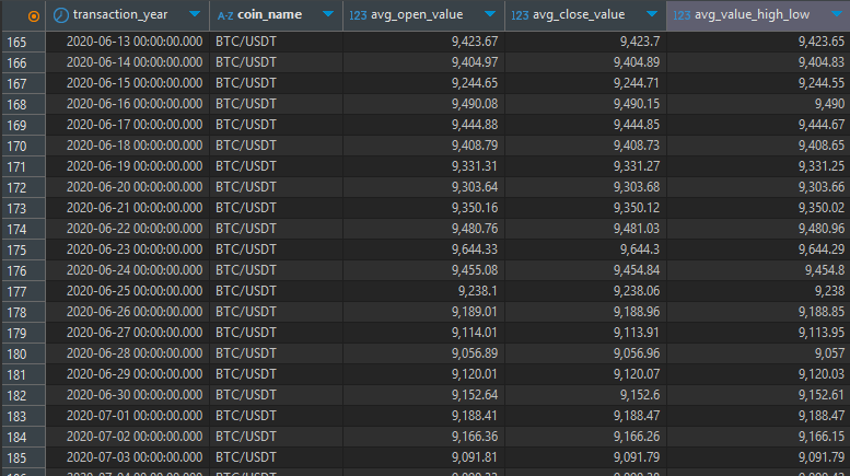
As seen in the examples, using time_bucket makes it very easy to group time.
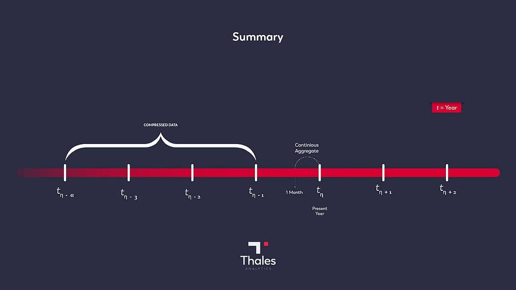
Compression and Continuous Aggregate Structures in TigerData
In TigerData, we can compress the part of the table before a certain time period on a hypertable. In Continuous Aggregate, we can convert the time period of the table into a materialized view and use it. The advantage of this on TigerData is that, for example, in a 7-day scenario, as data arrives in the table, the day range is preserved, and the data that falls to t-8 after the data arrives is automatically compressed, or the data remaining in the materialized view outside of 7 days is excluded from the view.
If we continue with our use case, I am using the coin_data table, which we assume to be very large 🙂 for forecasting analysis and reporting. For reporting, let’s assume that the data before 1 year is insignificant, and for analysis, it is sufficient that the train data is the last 1 month. In this context, we will compress the data before 1 year and the data of the last 1 month will always remain materialized. Since the training data will remain in memory, the analysis will be much faster.
Compression creation
ALTER TABLE coin_data SET (
  timescaledb.compress,
  timescaledb.compress_segmentby = 'symbol' ---for increased performance
);

SELECT add_compression_policy('coin_data', INTERVAL '1 year');Note: It is recommended to make these settings without inserting data into the table.
Creating a Continuous Aggregate
CREATE  MATERIALIZED VIEW tmp_schema.view_coin_data
WITH (timescaledb.continuous) as
select time_bucket('1 minute',transaction_time),transaction_time,symbol,
open_value, high_value, low_value, close_value, volume_coin, volume_usdt,
trade_count
from tmp_schema.coin_data
order by 1,2;

SELECT add_continuous_aggregate_policy('tmp_schema.view_coin_data',
  start_offset => interval '1 month', ---Updating timeframe first day: 1 month from now
  end_offset => null , ---Updating timeframe last day: now
schedule_interval => INTERVAL '1 Day' ---Run this update policy once a dayAs a result of all these improvements, the final version of our table is:
Conclusion
In TigerData, we used a very simple table creation, customization, compression, continuous aggregate and select writing features. In fact, many improvements can be made to increase performance, but we wanted to keep the article short. Let’s not think of TigerData as a database that works only on time series. It is actually a type of segmentation. So we can also make chunk assignments on words and get fast results this way. The fact that it works on a powerful and widespread product like PostgreSQL, if used with other plugins (pgvector, PostGIS, DuckDB, etc.), can create a very efficient structure for data warehouse and analytical work.